The Often Overlooked Consideration for Energy-Efficient Computing? Node Sizing.

There are constant arguments, opinions, and memes about how to make more sustainable decisions.
“Electric cars are the future!”
“But most EV batteries are composed of several rare earth minerals, including cobalt and lithium…”
“Okay, let’s jump to paper straws!”
“But 90% of paper straws were found to have concentrations of forever chemicals, known as poly- and perfluoroalkyl substances…”
While you have no direct say on the many manufacturing processes that affect sustainability, if you’re reading this, you are probably empowered to use more sustainable coding practices and make small but incredibly powerful decisions to change the trajectory of your code.
Computing resources are the building blocks for a movement towards energy efficiency and reducing our carbon footprint. So let’s start by talking about node sizing. How do you strike that sweet spot between size, performance, and cost from the get-go? With some of my experience over the years and a practical example, that’s exactly what we’re going to answer here.
Small Nodes Vs Big Nodes
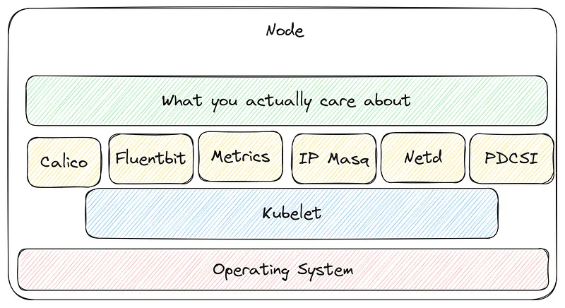
If we take the common case of Kubernetes, where our nodes are seen as a resource pool, each one of those nodes needs to dedicate a fraction of its resources to overhead.
Running a GKE cluster nowadays has the following Daemonsets (as an example):
kube-system   calico-node
kube-system   fluentbit-gke
kube-system   gke-metadata-server
kube-system   gke-metrics-agent
kube-system   ip-masq-agent
kube-system   netd
kube-system   pdcsi-node
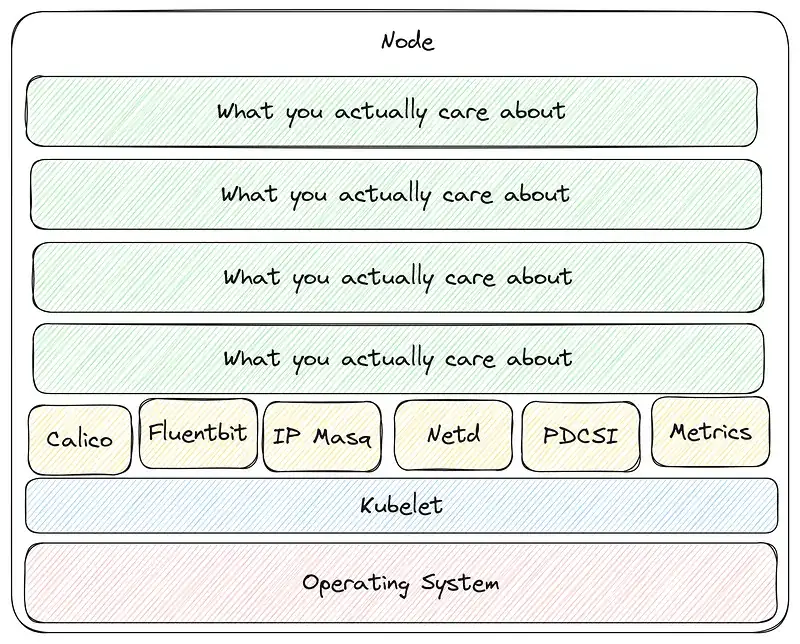
The above is a very minimal cluster with no special setup, each node is running seven pods to manage it, if you add the Kubelet and the operating system your nodes start looking pretty crowded (before you’re even running any workloads on it)
When this is running at scale that overhead will grow and your footprint grows with it.
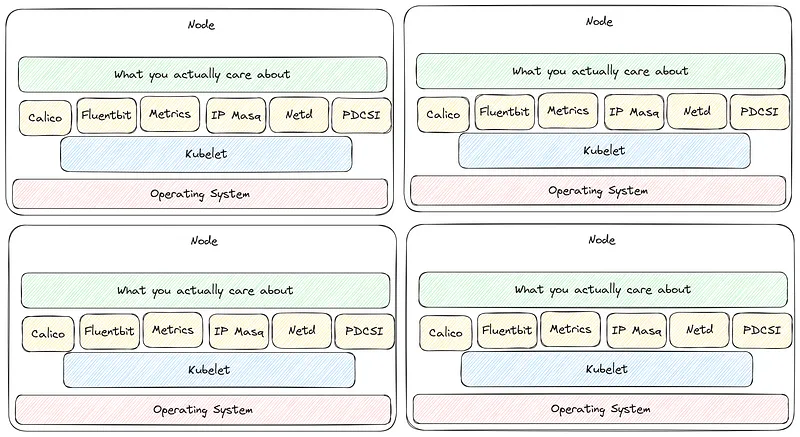
If we’re aiming to tune up our cloud setup for better efficiency, it’s time for a deep dive into our workloads. It’s not a plug-and-play situation; we’ve got to consider several key factors like:
- Size of the application — how much digital elbow room does it need to run without a hitch?
- The ‘noisy neighbor effect’ — we don’t want one app hogging all the resources.
- Scaling, which can be about stretching the node itself or the application, depending on the demand.
- The balancing act of managing peak usage times versus the quiet times.
When you toss cost considerations and the nitty-gritty of application architecture into the mix, you’ve got a pretty complex puzzle to solve. If you nail all these calculations, your system will start to shape up into something much more streamlined and energy-efficient like this:
What does this look like in practice?
I have set up a small demonstration using two clusters running the Google Microservices Demo.
Cluster one is running smaller nodes (2VCPU’s + 8GB RAM) while cluster two is running slightly bigger (double the size) nodes (4VCPU’s and 16GB)
I ran both of the clusters for two days to remove any variance caused by deployments etc.
Have a look at some of the findings:
Cluster Node Count While running the setup there is a notice that the application only needs two nodes to run in Cluster Two, while in Cluster One it needs three nodes.
Cluster One:
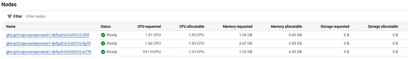
Cluster Two:

Something to note here is that on Cluster Two the nodes still have some processing power to spare, while the smaller nodes are running at maximum capacity (for CPU).
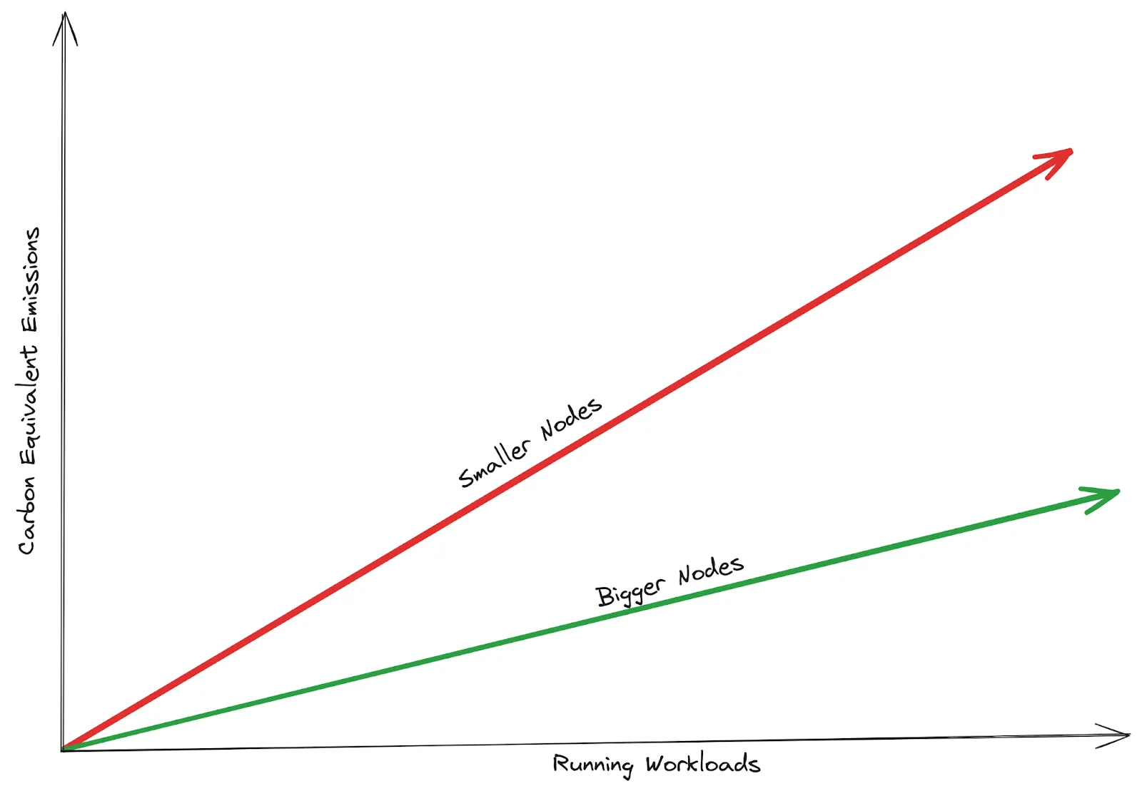
Carbon Efficiency When comparing the energy overhead of each cluster, by seeing the Carbon Footprint of the kube-system namespace (using kepler) in each cluster, we can quickly see that even though we are running the exact same workloads across both clusters, the cluster with the bigger nodes is using less carbon per day to run (while also having space to run even more workloads) than the smaller cluster:
Cluster One:

Cluster Two:

As we scale our workloads, this difference in emissions becomes more apparent
One last consideration is the idea of how utilised our nodes are. This also has an effect on carbon intensity and is known as “Energy Proportionality”.
Energy Proportionality
The concept of “Energy Proportionality” is becoming increasingly crucial for sustainable computing. The logic is simple yet profound: an idle server contributes no value to workload processing, but it consumes power. In contrast, a server operating at 50% capacity may consume more energy than one at idle, but it delivers significantly greater value. This value exponentially increases as we reach full utilisation; a server at full capacity may only require a fraction more energy than one at 50% load, yet it offers double the productivity.
Essentially, as server utilisation goes up, the rate at which power consumption increases slows down, making high-efficiency utilisation a smart strategy for both the environment and the bottom line.
This principle is a guiding light for businesses aiming to maximise output while minimising their energy footprint.
In conclusion…
Smaller doesn’t always mean less. While the flexibility and initial budget-friendliness of using smaller nodes are tempting, they easily lead to higher energy use, lower utilisation, and spiraling inefficiencies.
While this is not a call to just go for the biggest machines available to us, for now, the quickest way for earth-conscious IT practitioners to help reduce carbon emissions is to revisit our node size calculations in the past and see if we might be better off altering our machines to better reflect the value that we are creating.